What is a kernel function

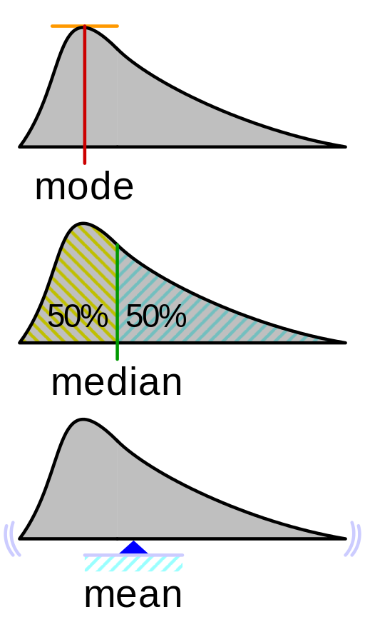
The Probability Density Function is a function that used to specify the possibility of a continous random variable falling within a particular range of values (as apposed to taking on any value). This probability is given by the area under the density function but above the horizontal axis and between the lowest and greatest values of the range. An example probability density function is as below:

And the Probability Density Function has the following properties:

• non-negative everywhere
• integral over the entire space is equal to 1
• real-valued (continuous)

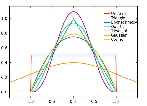
A kernel is a special type of Probability Density Function with the added property that it must be even. Some of the commonly used kernels are shown in the diagram below:

What is Kernel Density Estimation

Kernel Density Estimation is a non-parametric method for estimating the probability density function of a continuous random variable. non-parametric means that we are not assuming any underlying distribution for the random variable.

The way it works is as following. At every data point (datum), a kernel function is created with the data point at its centre. The probability density function for the continuous random variable is then estimated by adding all these kernel functions and dividing by the number of data points to ensure that the resulting probability density function meets the following requirements: - non-negative everywhere - the integral of the entire space is equal to 1

Intuitively, the Kernel Density Estimation method sums up the bumps and divides the resulting function by the number of bumps.

Each "bump" is centred at a data point and it speads out to cover the data point's neighbouring values. Each kernel has a bandwidth which determines the width of the bump. A bigger bandwidth results in a shorter and wider bump that spreads out farther from the centre and assigns more probability to the neighbouring values.

Steps to construct a Kernel Density Estimation

1. Choose a kernel such as mornal (Gaussian), uniform or triangular and decide the bandwidth (also called window width or the smoothing parameter).
2. Build a scaled kernel function for each data point.
3. Add all the kernel functions and dived by the number of kernel functions.

Choosing the bandwidth

Choosing the bandwidth turns out to be the most difficult step in creating a good kernel density estimate that captures the underlying distribution of the continuous random variable. We will need to review various literatures to decide on the best bandwidth. But below is a general guideline:

• A small bandwidth results in a small standard deviation, and the kernel places most of the probability on the data point. Use this when the training data is large and the data points are tightly packed.
• A large bandwidth results in a large standard deviation, and the kernel spreads more of the possibility from the data point to its neighbouring values. Use this when the training data is small and the data points are sparse.